9. Complex Numbers and Trigonometry#

9.1. Overview#

This lecture introduces some elementary mathematics and trigonometry.

Useful and interesting in its own right, these concepts reap substantial rewards when studying dynamics generated by linear difference equations or linear differential equations.

For example, these tools are keys to understanding outcomes attained by Paul Samuelson (1939) [Samuelson, 1939] in his classic paper on interactions between the investment accelerator and the Keynesian consumption function, our topic in the lecture Samuelson Multiplier Accelerator.

In addition to providing foundations for Samuelson’s work and extensions of it, this lecture can be read as a stand-alone quick reminder of key results from elementary high school trigonometry.

So let’s dive in.

9.1.1. Complex Numbers#

A complex number has a real part $x$ and a purely imaginary part $y$ .

The Euclidean, polar, and trigonometric forms of a complex number $z$ are:

z = x + i y = r e^{i θ} = r (\cos θ + i \sin θ)

The second equality above is known as Euler’s formula

Euler contributed many other formulas too!

The complex conjugate $\bar{z}$ of $z$ is defined as

\bar{z} = x - i y = r e^{- i θ} = r (\cos θ - i \sin θ)

The value $x$ is the real part of $z$ and $y$ is the imaginary part of $z$ .

The symbol $| z |$ = $\sqrt{\bar{z} \cdot z} = r$ represents the modulus of $z$ .

The value $r$ is the Euclidean distance of vector $(x, y)$ from the origin:

r = | z | = \sqrt{x^{2} + y^{2}}

The value $θ$ is the angle of $(x, y)$ with respect to the real axis.

Evidently, the tangent of $θ$ is $(\frac{y}{x})$ .

Therefore,

θ = \tan^{- 1} (\frac{y}{x})

Three elementary trigonometric functions are

\cos θ = \frac{x}{r} = \frac{e^{i θ} + e^{- i θ}}{2}, \sin θ = \frac{y}{r} = \frac{e^{i θ} - e^{- i θ}}{2 i}, \tan θ = \frac{y}{x}

We’ll need the following imports:

import matplotlib.pyplot as plt
plt.rcParams["figure.figsize"] = (11, 5)  #set default figure size
import numpy as np
from sympy import (Symbol, symbols, Eq, nsolve, sqrt, cos, sin, simplify,
                  init_printing, integrate)

9.1.2. An Example#

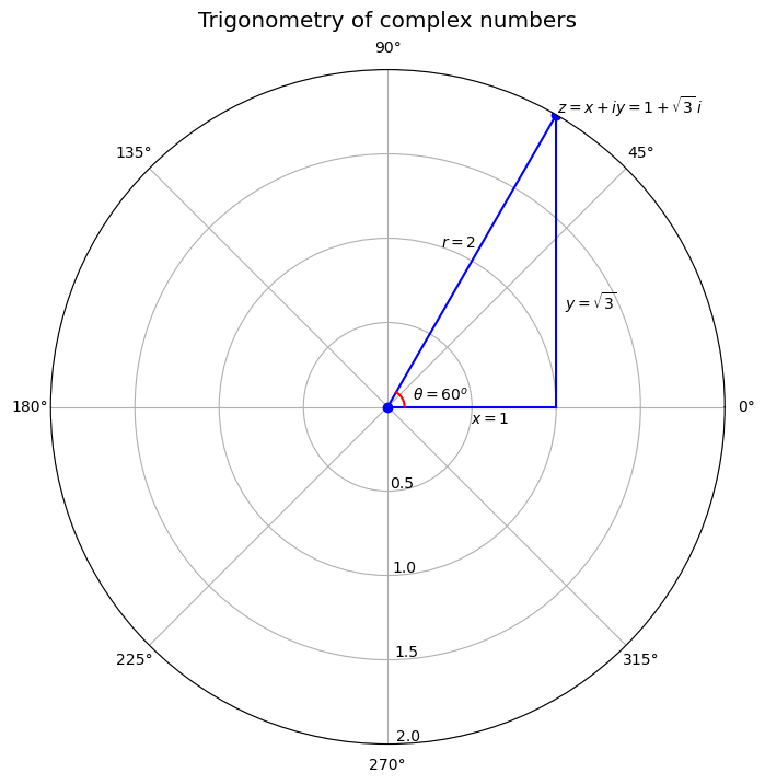
Example 9.1

Consider the complex number $z = 1 + \sqrt{3} i$ .

For $z = 1 + \sqrt{3} i$ , $x = 1$ , $y = \sqrt{3}$ .

It follows that $r = 2$ and $θ = \tan^{- 1} (\sqrt{3}) = \frac{π}{3} = 60^{o}$ .

Let’s use Python to plot the trigonometric form of the complex number $z = 1 + \sqrt{3} i$ .

# Abbreviate useful values and functions
π = np.pi


# Set parameters
r = 2
θ = π/3
x = r * np.cos(θ)
x_range = np.linspace(0, x, 1000)
θ_range = np.linspace(0, θ, 1000)

# Plot
fig = plt.figure(figsize=(8, 8))
ax = plt.subplot(111, projection='polar')

ax.plot((0, θ), (0, r), marker='o', color='b')          # Plot r
ax.plot(np.zeros(x_range.shape), x_range, color='b')       # Plot x
ax.plot(θ_range, x / np.cos(θ_range), color='b')        # Plot y
ax.plot(θ_range, np.full(θ_range.shape, 0.1), color='r')  # Plot θ

ax.margins(0) # Let the plot starts at origin

ax.set_title("Trigonometry of complex numbers", va='bottom',
    fontsize='x-large')

ax.set_rmax(2)
ax.set_rticks((0.5, 1, 1.5, 2))  # Less radial ticks
ax.set_rlabel_position(-88.5)    # Get radial labels away from plotted line

ax.text(θ, r+0.01 , r'$z = x + iy = 1 + \sqrt{3}\, i$')   # Label z
ax.text(θ+0.2, 1 , '$r = 2$')                             # Label r
ax.text(0-0.2, 0.5, '$x = 1$')                            # Label x
ax.text(0.5, 1.2, r'$y = \sqrt{3}$')                      # Label y
ax.text(0.25, 0.15, r'$\theta = 60^o$')                   # Label θ

ax.grid(True)
plt.show()

_images/c3e0ee881a15115309bc7dda9b1fb2f9022098f773ca979bfc42195dc1b1a7bf.png

9.2. De Moivre’s Theorem#

de Moivre’s theorem states that:

(r (\cos θ + i \sin θ))^{n} = r^{n} e^{i n θ} = r^{n} (\cos n θ + i \sin n θ)

To prove de Moivre’s theorem, note that

(r (\cos θ + i \sin θ))^{n} = (r e^{i θ})^{n}

and compute.

9.3. Applications of de Moivre’s Theorem#

9.3.1. Example 1#

We can use de Moivre’s theorem to show that $r = \sqrt{x^{2} + y^{2}}$ .

We have

\begin{array}{r} \begin{aligned} 1 & = e^{i θ} e^{- i θ} \\ = (\cos θ + i \sin θ) (\cos (- θ) + i \sin (- θ)) \\ = (\cos θ + i \sin θ) (\cos θ - i \sin θ) \\ = \cos^{2} θ + \sin^{2} θ \\ = \frac{x^{2}}{r^{2}} + \frac{y^{2}}{r^{2}} \end{aligned} \end{array}

and thus

x^{2} + y^{2} = r^{2}

We recognize this as a theorem of Pythagoras.

9.3.2. Example 2#

Let $z = r e^{i θ}$ and $\bar{z} = r e^{- i θ}$ so that $\bar{z}$ is the complex conjugate of $z$ .

$(z, \bar{z})$ form a complex conjugate pair of complex numbers.

Let $a = p e^{i ω}$ and $\bar{a} = p e^{- i ω}$ be another complex conjugate pair.

For each element of a sequence of integers $n = 0, 1, 2, \dots,$ .

To do so, we can apply de Moivre’s formula.

Thus,

\begin{array}{r} \begin{aligned} x_{n} & = a z^{n} + \bar{a} {\bar{z}}^{n} \\ = p e^{i ω} (r e^{i θ})^{n} + p e^{- i ω} (r e^{- i θ})^{n} \\ = p r^{n} e^{i (ω + n θ)} + p r^{n} e^{- i (ω + n θ)} \\ = p r^{n} [\cos (ω + n θ) + i \sin (ω + n θ) + \cos (ω + n θ) - i \sin (ω + n θ)] \\ = 2 p r^{n} \cos (ω + n θ) \end{aligned} \end{array}

9.3.3. Example 3#

This example provides machinery that is at the heard of Samuelson’s analysis of his multiplier-accelerator model [Samuelson, 1939].

Thus, consider a second-order linear difference equation

x_{n + 2} = c_{1} x_{n + 1} + c_{2} x_{n}

whose characteristic polynomial is

z^{2} - c_{1} z - c_{2} = 0

(z^{2} - c_{1} z - c_{2}) = (z - z_{1}) (z - z_{2}) = 0

has roots $z_{1}, z_{1}$ .

A solution is a sequence ${x_{n}}_{n = 0}^{\infty}$ that satisfies the difference equation.

Under the following circumstances, we can apply our example 2 formula to solve the difference equation

the roots $z_{1}, z_{2}$ of the characteristic polynomial of the difference equation form a complex conjugate pair
the values $x_{0}, x_{1}$ are given initial conditions

To solve the difference equation, recall from example 2 that

x_{n} = 2 p r^{n} \cos (ω + n θ)

where $ω, p$ are coefficients to be determined from information encoded in the initial conditions $x_{1}, x_{0}$ .

Since $x_{0} = 2 p \cos ω$ and $x_{1} = 2 p r \cos (ω + θ)$ the ratio of $x_{1}$ to $x_{0}$ is

\frac{x_{1}}{x_{0}} = \frac{r \cos (ω + θ)}{\cos ω}

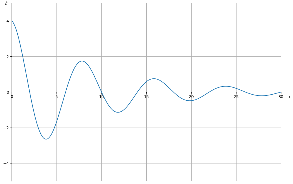
We can solve this equation for $ω$ then solve for $p$ using $x_{0} = 2 p r^{0} \cos (ω + n θ)$ .

With the sympy package in Python, we are able to solve and plot the dynamics of $x_{n}$ given different values of $n$ .

In this example, we set the initial values: - $r = 0.9$ - $θ = \frac{1}{4} π$ - $x_{0} = 4$ - $x_{1} = r \cdot 2 \sqrt{2} = 1.8 \sqrt{2}$ .

We first numerically solve for $ω$ and $p$ using nsolve in the sympy package based on the above initial condition:

# Set parameters
r = 0.9
θ = π/4
x0 = 4
x1 = 2 * r * sqrt(2)

# Define symbols to be calculated
ω, p = symbols('ω p', real=True)

# Solve for ω
## Note: we choose the solution near 0
eq1 = Eq(x1/x0 - r * cos(ω+θ) / cos(ω), 0)
ω = nsolve(eq1, ω, 0)
ω = float(ω)
print(f'ω = {ω:1.3f}')

# Solve for p
eq2 = Eq(x0 - 2 * p * cos(ω), 0)
p = nsolve(eq2, p, 0)
p = float(p)
print(f'p = {p:1.3f}')

ω = 0.000
p = 2.000

Using the code above, we compute that $ω = 0$ and $p = 2$ .

Then we plug in the values we solve for $ω$ and $p$ and plot the dynamic.

# Define range of n
max_n = 30
n = np.arange(0, max_n+1, 0.01)

# Define x_n
x = lambda n: 2 * p * r**n * np.cos(ω + n * θ)

# Plot
fig, ax = plt.subplots(figsize=(12, 8))

ax.plot(n, x(n))
ax.set(xlim=(0, max_n), ylim=(-5, 5), xlabel='$n$', ylabel='$x_n$')

# Set x-axis in the middle of the plot
ax.spines['bottom'].set_position('center')
ax.spines['right'].set_color('none')
ax.spines['top'].set_color('none')
ax.xaxis.set_ticks_position('bottom')
ax.yaxis.set_ticks_position('left')

ticklab = ax.xaxis.get_ticklabels()[0] # Set x-label position
trans = ticklab.get_transform()
ax.xaxis.set_label_coords(31, 0, transform=trans)

ticklab = ax.yaxis.get_ticklabels()[0] # Set y-label position
trans = ticklab.get_transform()
ax.yaxis.set_label_coords(0, 5, transform=trans)

ax.grid()
plt.show()

_images/2047be876c84e7faed97f85602b06cb65570c7013d34fd9e749a53882c9a4539.png

9.3.4. Trigonometric Identities#

We can obtain a complete suite of trigonometric identities by appropriately manipulating polar forms of complex numbers.

We’ll get many of them by deducing implications of the equality

e^{i (ω + θ)} = e^{i ω} e^{i θ}

For example, we’ll calculate identities for

$\cos (ω + θ)$ and $\sin (ω + θ)$ .

Using the sine and cosine formulas presented at the beginning of this lecture, we have:

\begin{array}{r} \begin{matrix} \cos (ω + θ) = \frac{e^{i (ω + θ)} + e^{- i (ω + θ)}}{2} \\ \sin (ω + θ) = \frac{e^{i (ω + θ)} - e^{- i (ω + θ)}}{2 i} \end{matrix} \end{array}

We can also obtain the trigonometric identities as follows:

\begin{array}{r} \begin{aligned} \cos (ω + θ) + i \sin (ω + θ) & = e^{i (ω + θ)} \\ = e^{i ω} e^{i θ} \\ = (\cos ω + i \sin ω) (\cos θ + i \sin θ) \\ = (\cos ω \cos θ - \sin ω \sin θ) + i (\cos ω \sin θ + \sin ω \cos θ) \end{aligned} \end{array}

Since both real and imaginary parts of the above formula should be equal, we get:

\begin{array}{r} \begin{matrix} \cos (ω + θ) = \cos ω \cos θ - \sin ω \sin θ \\ \sin (ω + θ) = \cos ω \sin θ + \sin ω \cos θ \end{matrix} \end{array}

The equations above are also known as the angle sum identities. We can verify the equations using the simplify function in the sympy package:

# Define symbols
ω, θ = symbols('ω θ', real=True)

# Verify
print("cos(ω)cos(θ) - sin(ω)sin(θ) =",
    simplify(cos(ω)*cos(θ) - sin(ω) * sin(θ)))
print("cos(ω)sin(θ) + sin(ω)cos(θ) =",
    simplify(cos(ω)*sin(θ) + sin(ω) * cos(θ)))

cos(ω)cos(θ) - sin(ω)sin(θ) = cos(θ + ω)
cos(ω)sin(θ) + sin(ω)cos(θ) = sin(θ + ω)

9.3.5. Trigonometric Integrals#

We can also compute the trigonometric integrals using polar forms of complex numbers.

For example, we want to solve the following integral:

\int_{- π}^{π} \cos (ω) \sin (ω) d ω

Using Euler’s formula, we have:

\begin{array}{r} \begin{aligned} \int \cos (ω) \sin (ω) d ω & = \int \frac{(e^{i ω} + e^{- i ω})}{2} \frac{(e^{i ω} - e^{- i ω})}{2 i} d ω \\ = \frac{1}{4 i} \int e^{2 i ω} - e^{- 2 i ω} d ω \\ = \frac{1}{4 i} (\frac{- i}{2} e^{2 i ω} - \frac{i}{2} e^{- 2 i ω} + C_{1}) \\ = - \frac{1}{8} [(e^{i ω})^{2} + (e^{- i ω})^{2} - 2] + C_{2} \\ = - \frac{1}{8} (e^{i ω} - e^{- i ω})^{2} + C_{2} \\ = \frac{1}{2} (\frac{e^{i ω} - e^{- i ω}}{2 i})^{2} + C_{2} \\ = \frac{1}{2} \sin^{2} (ω) + C_{2} \end{aligned} \end{array}

and thus:

\int_{- π}^{π} \cos (ω) \sin (ω) d ω = \frac{1}{2} \sin^{2} (π) - \frac{1}{2} \sin^{2} (- π) = 0

We can verify the analytical as well as numerical results using integrate in the sympy package:

# Set initial printing
init_printing(use_latex="mathjax")

ω = Symbol('ω')
print('The analytical solution for integral of cos(ω)sin(ω) is:')
integrate(cos(ω) * sin(ω), ω)

The analytical solution for integral of cos(ω)sin(ω) is:

\frac{\sin^{2} (ω)}{2}

print('The numerical solution for the integral of cos(ω)sin(ω) \
from -π to π is:')
integrate(cos(ω) * sin(ω), (ω, -π, π))

The numerical solution for the integral of cos(ω)sin(ω) from -π to π is:

0

9.3.6. Exercises#

Exercise 9.1

We invite the reader to verify analytically and with the sympy package the following two equalities:

\int_{- π}^{π} \cos (ω)^{2} d ω = π

\int_{- π}^{π} \sin (ω)^{2} d ω = π

Solution to Exercise 9.1

Let’s import symbolic $π$ from sympy

# Import symbolic π from sympy
from sympy import pi

print('The analytical solution for the integral of cos(ω)**2 \
from -π to π is:')

integrate(cos(ω)**2, (ω, -pi, pi))

The analytical solution for the integral of cos(ω)**2 from -π to π is:

π

print('The analytical solution for the integral of sin(ω)**2 \
from -π to π is:')

integrate(sin(ω)**2, (ω, -pi, pi))

The analytical solution for the integral of sin(ω)**2 from -π to π is:

π